Summary

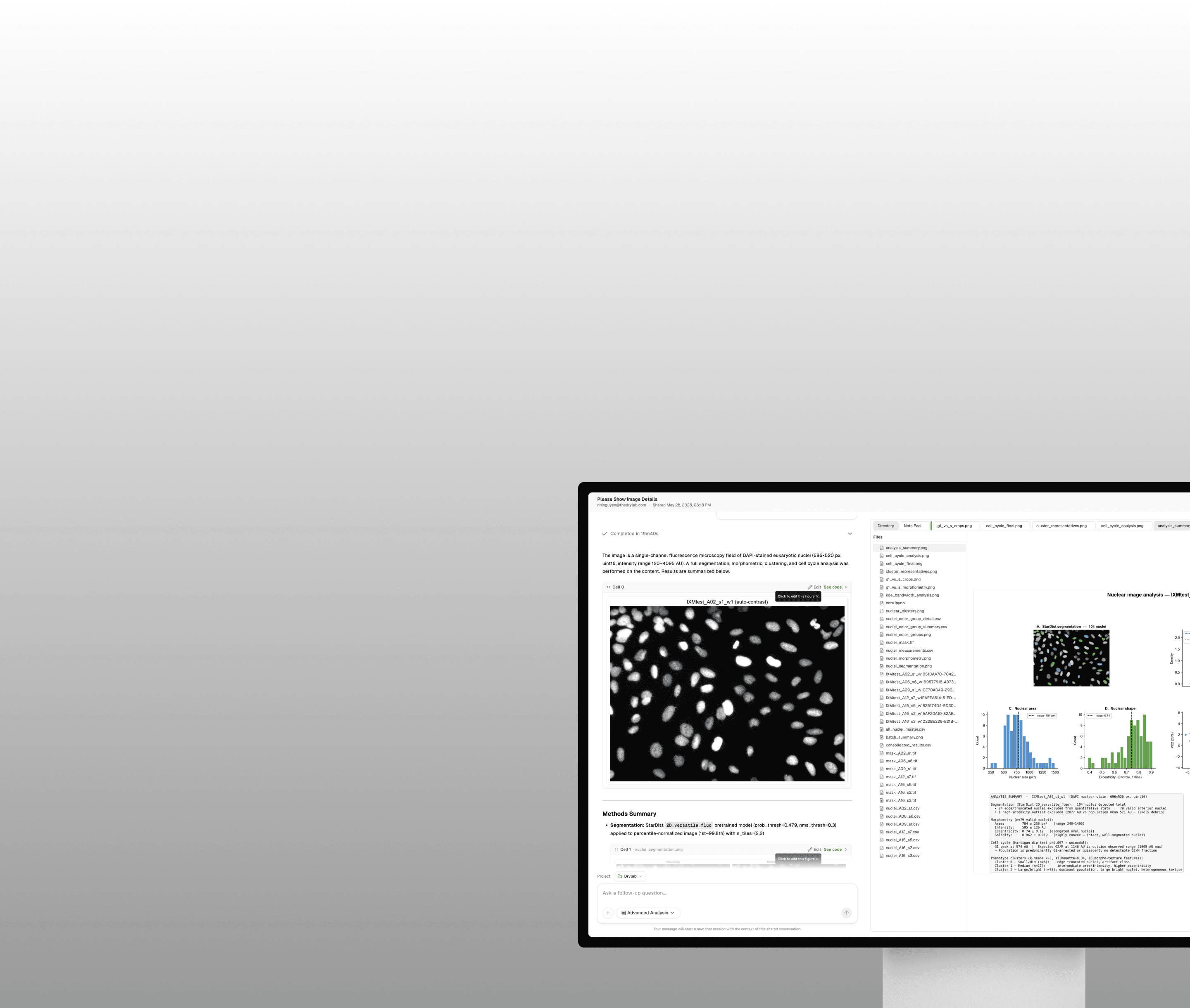
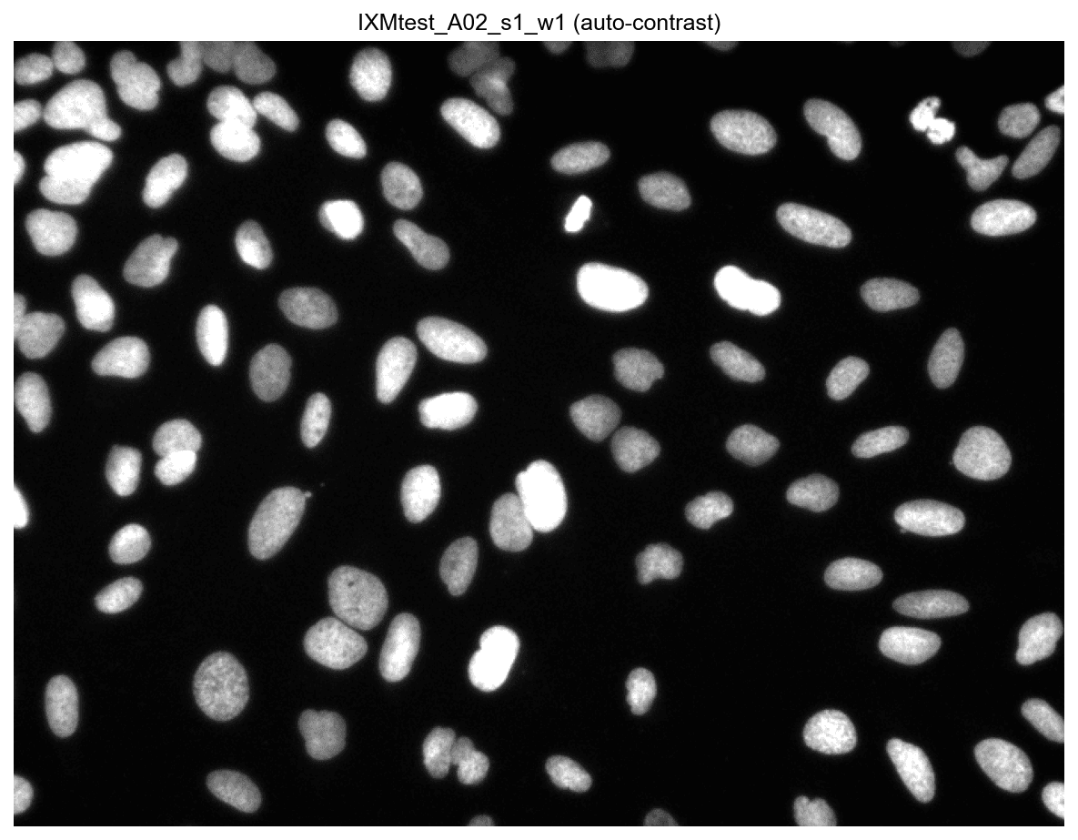
Analyze DAPI-stained microscopy images to identify individual nuclei, quantify nuclear morphology, and estimate cell cycle states based on DNA content and chromatin organization. The workflow combines automated nuclear segmentation with single-cell morphometric and texture analysis to characterize cell populations.

Input

DAPI-stained fluorescence microscopy images

Output

• Nuclear segmentation masks

• Cell count per image

• Nuclear size and morphology measurements

• Cell cycle phase classification (G1, S, G2/M)

• Chromatin texture features

• Population-level summary statistics and visualizations

Analysis breakdown

1. Segmentation & QC

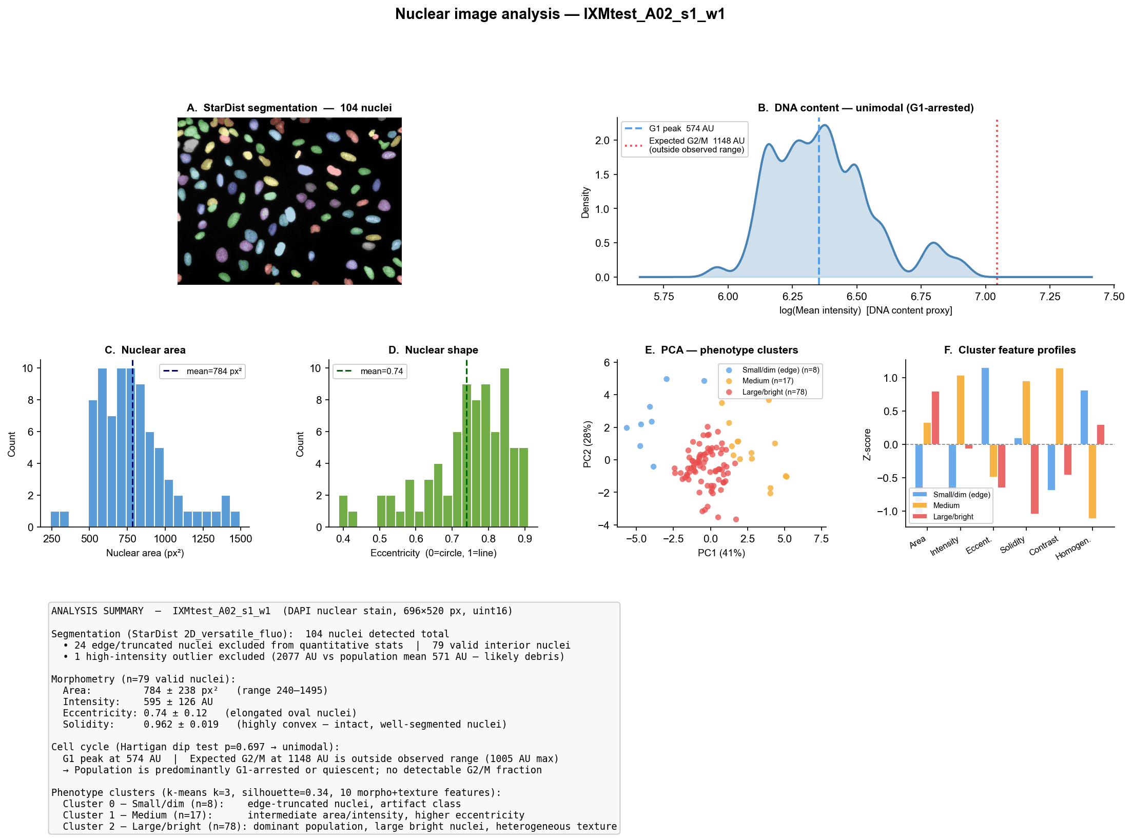
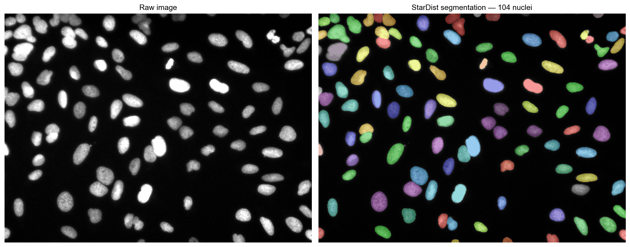
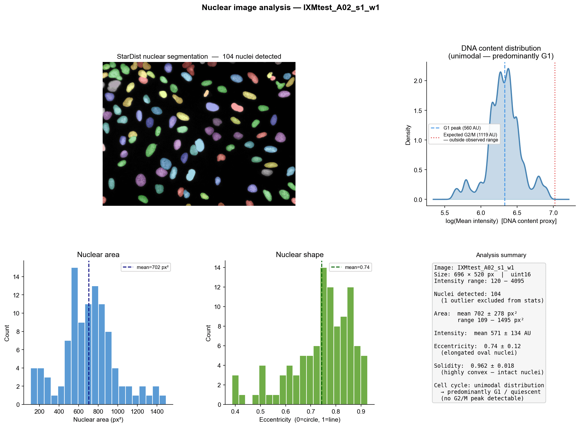
StarDist 2D_versatile_fluo pretrained model (prob_thresh=0.479, nms_thresh=0.3) applied to percentile-normalized image (1st–99.8th) with n_tiles=(2,2)

• StarDist detected 104 nuclei total; 1 high-intensity outlier (2,077 AU vs population mean 571 AU — likely debris) excluded

• 24 nuclei flagged as edge-truncated (bounding box within 5 px of image border); final valid cohort: 79 nuclei

  

  
  

2. Nuclear morphometry

(n=79 valid nuclei)

Morphometry: skimage.measure.regionprops_table — area, mean/max intensity, eccentricity, solidity, perimeter, centroid per nucleus

Texture: Haralick GLCM features (contrast, homogeneity, energy, correlation) at distance=1, four angles, 64 grey levels

• Area: mean 702 ± 280 px², range 109–1,495 px²

• Mean intensity: 571 ± 134 AU (population of 103, excl. outlier)

• Eccentricity: mean 0.744 (elongated ovals; 0=circle, 1=line)

• Solidity: mean 0.962 (highly convex — intact, well-segmented nuclei)

3. Clustering

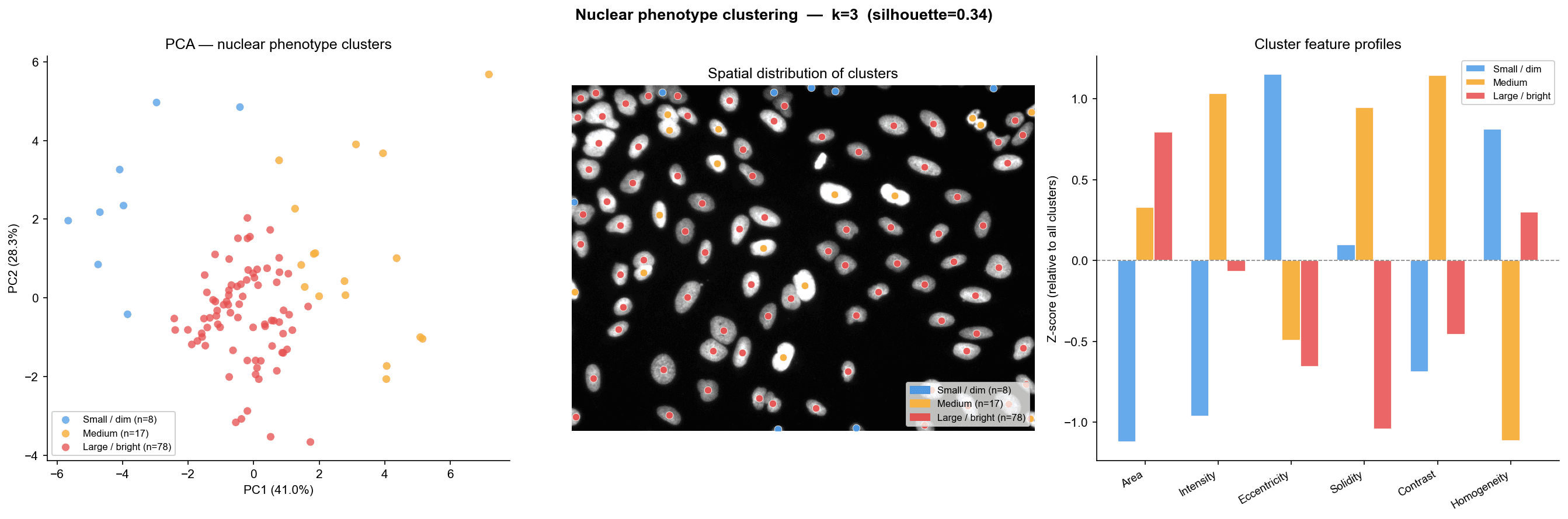
Unsupervised phenotypic clustering: KMeans (k=3, chosen by silhouette sweep k=2–6; silhouette=0.34) on 10 standardized morpho+texture features

Cluster 0 corresponds entirely to edge-truncated artifacts. The PCA space (PC1+PC2 = 69.3% variance) shows clear separation between clusters

Clusters 1 and 2 represent biologically distinct nuclear states — the dominant population (Cluster 2, n=78) comprises large, bright, highly convex nuclei consistent with interphase cells in G1, while the medium cluster (Cluster 1, n=17) captures nuclei with elevated intensity (781 vs 547 AU), higher texture contrast, and lower homogeneity, segregating into the S-phase fraction

4. Cell cycle

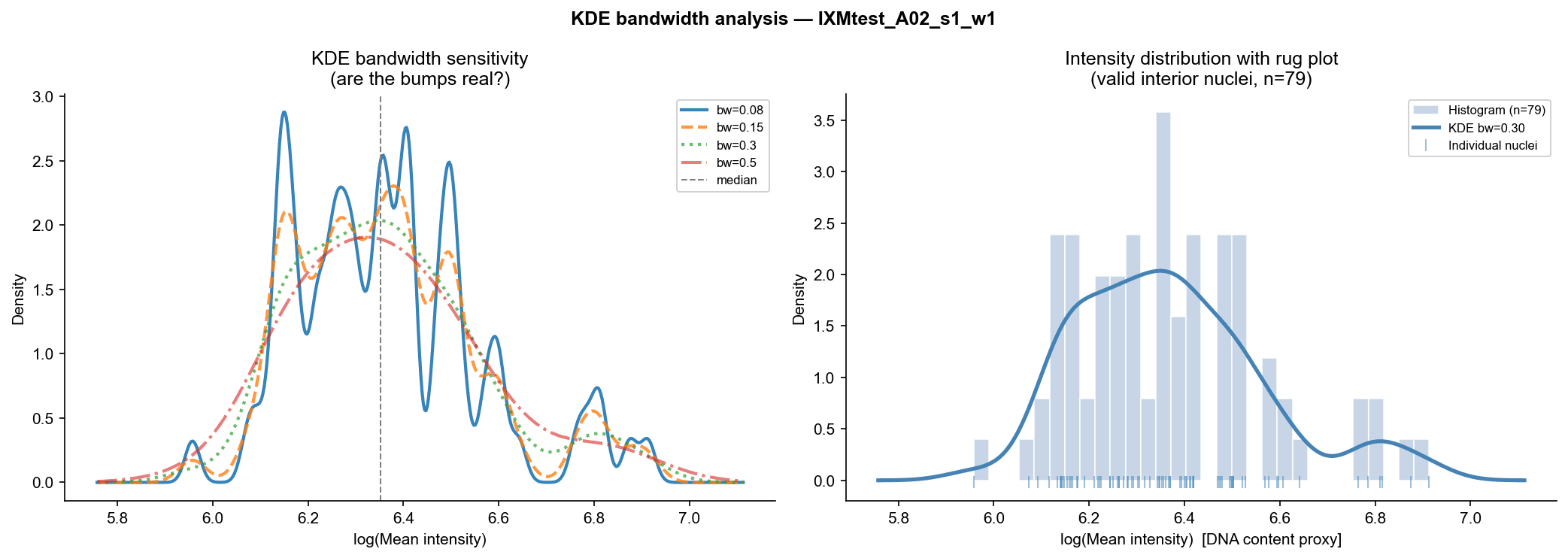
   The intensity distribution is formally unimodal (Hartigan p=0.697) and the absence of any G2/M nuclei — where none reached the expected 2× G1 DNA content threshold of ~1,100 AU — is consistent with a non-cycling, quiescent, or early-passage culture

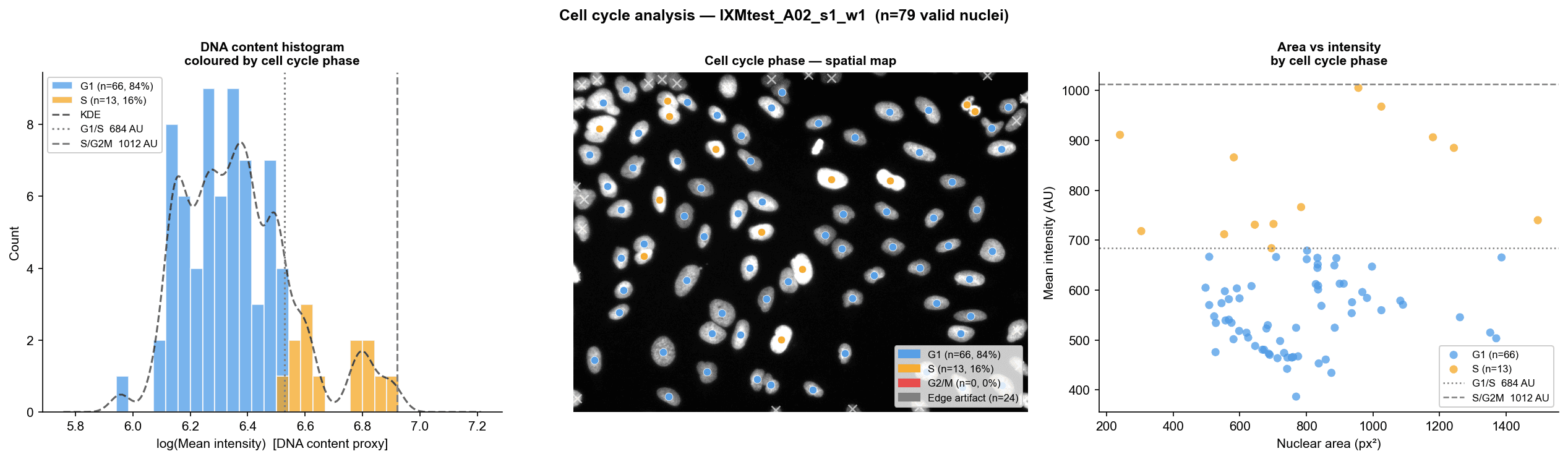
   • G1 baseline (dominant cluster median): 550 AU; expected G2/M at 2×G1 = 1,100 AU exceeds observed maximum (1,005 AU)

   • A minor S-phase fraction of 16.5% (n=12) is detectable via an intermediate intensity shoulder in the KDE at bw=0.15

• Biologically-informed thresholds: G1/S = 688 AU (1.25×); S/G2M = 1,018 AU (1.85×)

• G1: 67 nuclei (83.5%) | S-phase: 12 nuclei (16.5%) | G2/M: 0

5. G1 vs S comparison

G1 vs S-phase comparison (Mann-Whitney U, two-sided)

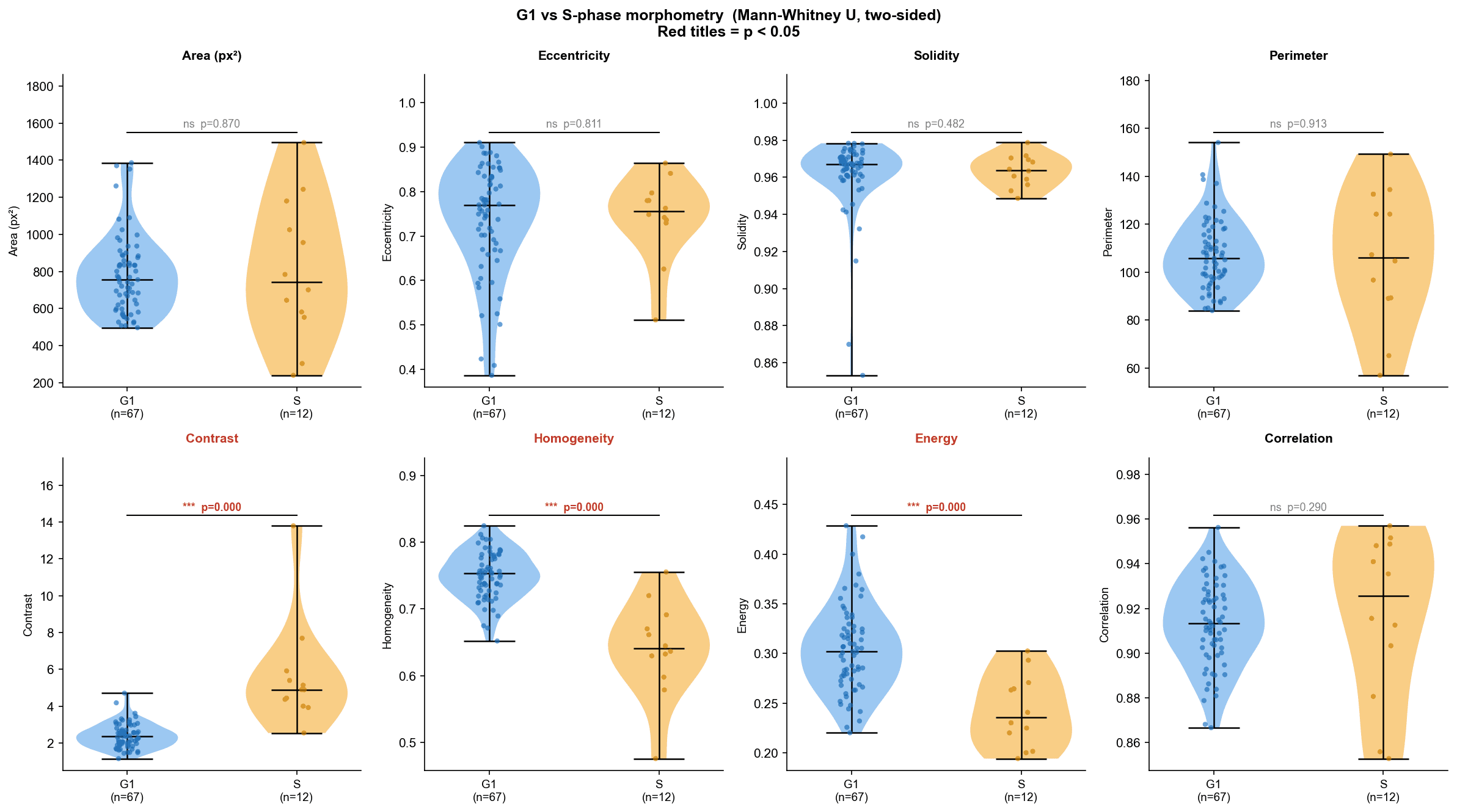
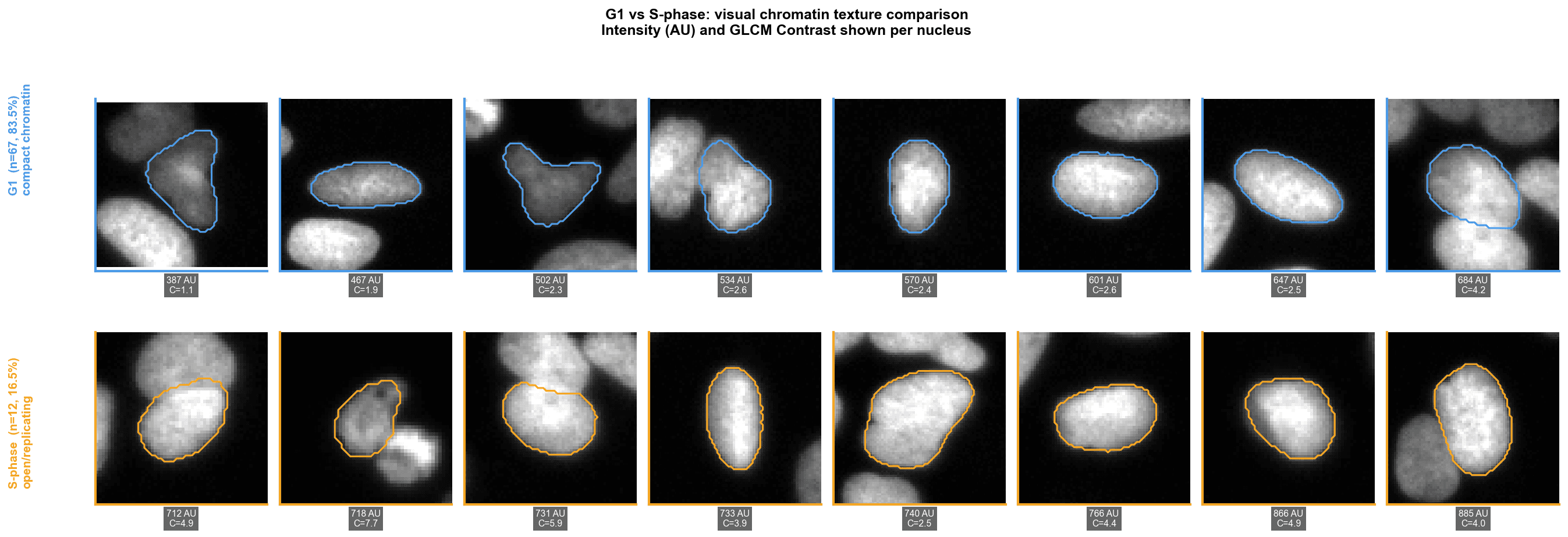
Chromatin texture as a phase discriminator: S-phase nuclei are morphometrically indistinguishable from G1 nuclei in size, shape, and perimeter (all Mann-Whitney p > 0.05), but exhibit a strong chromatin texture signature — 2.07-fold higher GLCM contrast (p=4.5e-7), lower homogeneity (fold=0.85, p=2.7e-6), and lower energy (fold=0.78, p=6.1e-5). This texture fingerprint is consistent with open, replication-fork chromatin architecture, where locally decondensed domains generate elevated pixel-to-pixel intensity variance (contrast) and disrupt the uniform, tightly packed texture of G1 heterochromatin (homogeneity and energy)

The visual crop gallery directly confirms these differences — S-phase nuclei show visibly grainier internal structure relative to the smoother G1 nuclei at comparable sizes

Standardize pipeline & Scale across multiple images

679 nuclei detected across 7 IXM fields; 549 valid nuclei retained after edge and outlier filtering

The three-panel summary figure below shows per-field nucleus counts by phase, S-phase fractions with cross-field mean, and GLCM contrast (G1 vs S) side-by-side.

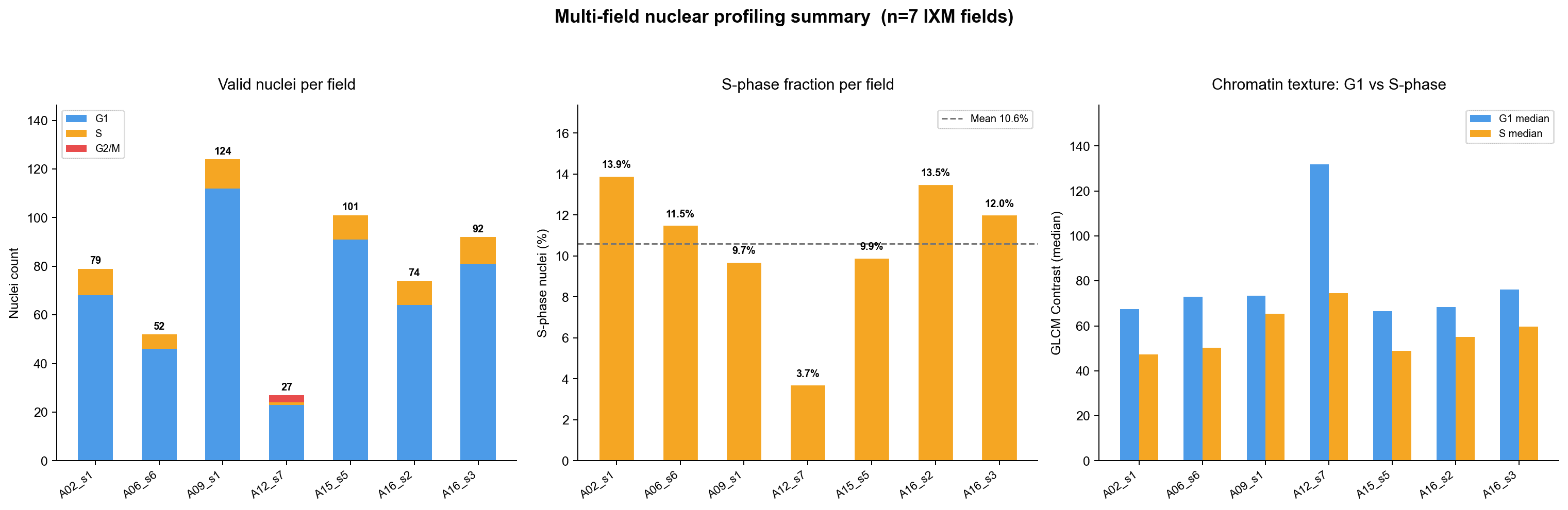
Cell counts: Valid nuclei per field range from 27 (A12_s7, a sparse field) to 124 (A09_s1). The 123 edge-artifact exclusions (18.1% of all detections) are uniform across fields, indicating consistent boundary effects expected for well-plate imaging.

• S-phase fraction: Consistent across six of seven fields at a mean of 10.6% ± 3.4% SD, compatible with an asynchronous, slow-cycling population.

• A12_s7 outlier: S-phase fraction drops to 3.7% (n=1) while G2/M rises to 11.1% (n=3) — the only field with detectable G2/M nuclei.

• GLCM contrast: G1 baseline contrast (median 79.5 AU) exceeds S-phase contrast (57.3 AU) consistently across all 7 fields, with per-field S/G1 ratios ranging 0.56–0.89×.